20 Linear Regression
20.1 Introduction
Regression plays a key part in modern-day statistics. R has advanced regression
functions that includes; lm() (for fitting linear models), glm() (for fitting
generalized linear models), nls() (for fitting nonlinear models) and coxph()
(for fitting a Cox proportional hazards regression model).
In statistical analysis, it often arises that the relationship between two continuous variables be expressed as a rate of rise per each unit of the other. For instance, one can ask:
On average, how many units of rise in the blood hematocrit occurs for each unit rise in blood haemoglobin content?
Readers who are conversant with this may guess the answer to be approximately 3.
20.2 Regression with single continuous independent variable
The basic idea behind linear regression is to have a formula where our dependent variable can be derived from our independent variable(s). Simply put if I am given one’s hb can I predict the person’s hct? To do this we come up with a formula for the form \[Y = aX + b\] Where \(Y\) is the dependent variable (hct), \(a\) is the slope of the straight line we draw through the points, \(X\) is the independent variable (hb) and \(b\) is the intercept or value of \(Y\) if \(a\) is 0.
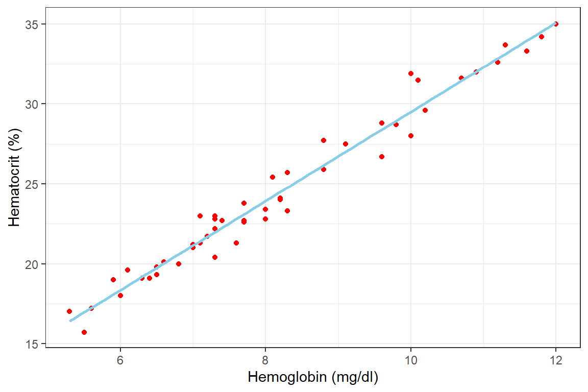
The first logical step in regression analysis is to plot a scatter diagram to visualize the relationship between the two variables. A plot of the hct versus the hb is shown below after importing the data
df_blood <- read_csv("./Data/blood.csv")And then summarize the data below
df_blood %>% summarytools::dfSummary(graph.col = F)
Data Frame Summary
df_blood
Dimensions: 50 x 7
Duplicates: 0

--------------------------------------------------------------------------------------
No   Variable    Stats / Values              Freqs (% of Valid)   Valid      Missing
---- ----------- --------------------------- -------------------- ---------- ---------
1    stno        Mean (sd) : 1025.5 (14.6)   50 distinct values   50         0
     [numeric]   min < med < max:                                 (100.0%)   (0.0%)
                 1001 < 1025.5 < 1050
                 IQR (CV) : 24.5 (0)

2    age         Mean (sd) : 122.4 (30.7)    19 distinct values   50         0
     [numeric]   min < med < max:                                 (100.0%)   (0.0%)
                 72 < 132 < 180
                 IQR (CV) : 48 (0.3)

3    wgt         Mean (sd) : 27.4 (7.7)      42 distinct values   50         0
     [numeric]   min < med < max:                                 (100.0%)   (0.0%)
                 17 < 26.3 < 59.5
                 IQR (CV) : 7.9 (0.3)

4    hgt         Mean (sd) : 130.5 (11.4)    27 distinct values   50         0
     [numeric]   min < med < max:                                 (100.0%)   (0.0%)
                 107 < 130.5 < 155
                 IQR (CV) : 15 (0.1)

5    hb          Mean (sd) : 8.2 (1.8)       36 distinct values   50         0
     [numeric]   min < med < max:                                 (100.0%)   (0.0%)
                 5.3 < 7.7 < 12
                 IQR (CV) : 2.6 (0.2)

6    wbc         Mean (sd) : 13.9 (8.8)      44 distinct values   50         0
     [numeric]   min < med < max:                                 (100.0%)   (0.0%)
                 4.8 < 11.4 < 62.6
                 IQR (CV) : 5.7 (0.6)

7    hct         Mean (sd) : 24.4 (5.1)      45 distinct values   50         0
     [numeric]   min < med < max:                                 (100.0%)   (0.0%)
                 15.7 < 23 < 35
                 IQR (CV) : 7.4 (0.2)
--------------------------------------------------------------------------------------
df_blood %>%
    ggplot(aes(x = hb, y = hct)) +
    geom_point(color = "red",)+
    geom_smooth(method = "lm", formula = y~x, color = "skyblue", se = F)+
    labs(x = "Hemoglobin (mg/dl)", y = "Hematocrit (%)") +
    theme_bw()
We now derive these constants with the lm() function as below.
| term | estimate | std.error | statistic | p.value | conf.low | conf.high |
|---|---|---|---|---|---|---|
| (Intercept) | 1.63 | 0.599 | 2.71 | 0.00921 | 0.421 | 2.83 |
| hb | 2.79 | 0.0716 | 39 | 5.53e-38 | 2.64 | 2.93 |
The table above gives us the values of the intercept (b) as 1.625 and the slope (a) as 2.778. We can thus say that based on our data there is an increase of approximately 2.788 in hematocrit for each unit rise in Hb. Also, the hct of the person with a Hb of 0 (if there is anything like it) will be 1.625. However, it is never a good idea to extrapolate this formula beyond the range of the data at hand. For instance, predicting the hct of anyone with an hb of 200 is not statistically and common sensically right.
Conclusion: For each unit rise in blood hb the hematocrit rises by about 2.8% in our sample. Extrapolating this onto the general population we are 95% certain that this rate of rise will fall between 2.6% and 2.9%. This observed slope is significantly different from a slope of 0. This is evident by the small p-value (<.001).
20.3 Regression with single categorical independent variable
Previously we implemented linear regression with one continuous independent variable. Here we implement linear regression with a categorical independent variable. In the blood data set, we do not have a categorical variable but we generate one by categorising those with high wbc (>11.0 x 10⁹/ml) as “High” and the others as “Low”.
df_blood <-
    df_blood %>%
    mutate(wbc.cat = case_when(wbc > 11 ~ "High", TRUE ~ "Low") %>%
               factor(levels=c("Low","High")))

df_blood %>% head()| stno | age | wgt | hgt | hb | wbc | hct | wbc.cat |
|---|---|---|---|---|---|---|---|
| 1e+03 | 120 | 18.4 | 128 | 7.7 | 13.7 | 22.6 | High |
| 1e+03 | 96 | 24 | 123 | 8 | 8.5 | 22.8 | Low |
| 1e+03 | 168 | 38.5 | 143 | 8.2 | 26.8 | 24.1 | High |
| 1e+03 | 96 | 20.4 | 114 | 8.3 | 10.5 | 23.3 | Low |
| 1e+03 | 132 | 26.9 | 132 | 7.3 | 10.7 | 22.2 | Low |
| 1.01e+03 | 108 | 26.8 | 131 | 6.8 | 9.7 | 20 | Low |
Next, we implement the linear regression
| term | estimate | std.error | statistic | p.value | conf.low | conf.high |
|---|---|---|---|---|---|---|
| (Intercept) | 27.1 | 0.973 | 27.8 | 3.02e-31 | 25.1 | 29 |
| wbc.catHigh | -4.7 | 1.3 | -3.62 | 0.000713 | -7.32 | -2.09 |
The interpretation here is slightly different from that with a single continuous variable.
- The estimate for the
(Intercept)is the mean of the hct at the lower level of the wbc.cat i.e. for those with wbc categorised as “Low”. The mean hct for those with “Low” wbc therefore is 27.055. - The coefficient
wbc.catHighis the difference between the mean hct of those with “High” and “Low” wbc.cat categories. Therefore the difference in mean hct for those with “High” and “Low” wbcs is -4.705. - The mean of the hct for those with “High” wbc.cat is the therefore
(Intercept)plus the coefficient of thewbc.catHigh. That is \(27.055 + (-4:405) = 22:35\).
For comparative purposes, we perform the analysis with the t.test() function below:
| estimate | estimate1 | estimate2 | statistic | p.value | parameter | conf.low | conf.high | method | alternative |
|---|---|---|---|---|---|---|---|---|---|
| 4.7 | 27.1 | 22.4 | 3.62 | 0.000713 | 48 | 2.09 | 7.32 | Two Sample t-test | two.sided |
A close look shows the two analyses produce identical results. The t-statistic,
p-value, 95% confidence interval of the difference and the sample estimates are
all identical. The question then arises: If we can easily derive this from the
t.test() function why go through this hassle of fitting a linear regression
model? The reason is regression opens a whole new world in statistics without
which many manipulations will be very difficult if not impossible to achieve.
Conclusion: The mean hct for those with “Low” wbc.cat is 27.0 with a 95% confidence interval of (25.1 to 29.0). The difference in hct between those with “High” and “Low” wbc is -4.7 with a 95% confidence interval of (-7.3 to -2.1). The difference between the two means is significantly different from 0 with a p-value = 0.001.
20.4 Regression with two continuous independent variables
Previously we have dealt with identifying and reporting a confounder or confounding in categorical data analysis. The effect used then was the odds ratio. In this subsection, we deal with confounding in linear regression using the regression coefficient often represented by \(\beta\) as the effect.
Previously we have identified a significant linear relationship between the blood hb and hct. For illustrative purposes, we present it again but show just the coefficients, their confidence interval and p-values.
| term | estimate | std.error | statistic | p.value | conf.low | conf.high |
|---|---|---|---|---|---|---|
| (Intercept) | 1.63 | 0.599 | 2.71 | 0.00921 | 0.421 | 2.83 |
| hb | 2.79 | 0.0716 | 39 | 5.53e-38 | 2.64 | 2.93 |
The output above shows a significant relationship between hb and hct (\(\beta\) = 2.778, 95%CI: 2.644 to 2.932, p=<.001). Previously, we learned that a confounder should be related to both the outcome and exposure variable. In our preliminary analysis, we decided to see if wbc is also related to the hct. This is done below
| term | estimate | std.error | statistic | p.value | conf.low | conf.high |
|---|---|---|---|---|---|---|
| (Intercept) | 28 | 1.23 | 22.8 | 2.24e-27 | 25.5 | 30.4 |
| wbc | -0.255 | 0.075 | -3.4 | 0.00137 | -0.405 | -0.104 |
Interestingly it appears so. There seems to be a significant reduction in wbc count with increasing hct. The question then arises:
Is the effect of the wbc being confounded by that of the hb?
To begin to investigate this we must first check if wbc has a relationship with the hb as well. This is done below
| term | estimate | std.error | statistic | p.value | conf.low | conf.high |
|---|---|---|---|---|---|---|
| (Intercept) | 31.6 | 5.3 | 5.97 | 2.76e-07 | 21 | 42.3 |
| hb | -2.17 | 0.633 | -3.43 | 0.00123 | -3.45 | -0.902 |
The result above indicates a significant reduction in wbc with increasing hb. By this result, we have demonstrated the relationship between three variables necessary for confounding to exist.
Next, we determine the adjusted coefficients for comparison to the crude ones. To do so we put both variables as independent variables in the linear regression formula as below
| term | estimate | std.error | statistic | p.value | conf.low | conf.high |
|---|---|---|---|---|---|---|
| (Intercept) | 1.69 | 0.799 | 2.12 | 0.0393 | 0.087 | 3.3 |
| hb | 2.78 | 0.0807 | 34.5 | 5.03e-35 | 2.62 | 2.95 |
| wbc | -0.00218 | 0.0165 | -0.132 | 0.895 | -0.0353 | 0.031 |
Both coefficients generated above (hb and wbc) are adjusted for each other. First we compare the crude effect of hb (\(\beta\) = 2.778, 95%CI: 2.644 to 2.932, p<.001) to the adjusted effect (\(\beta\) = 2.783, 95%CI: 2.621 to 2.946, p<.001). It is obvious there is literally no confounding of the relationship between hb and hct by wbc because the coefficient remains literally the same.
Next, we compare the crude relationship between wbc and hct (\(\beta\) = -0.255, 95%CI: -0.405 to -0.104, p=0.001) to the adjusted relationship (\(\beta\) = -0.002, 95%CI: -0.035 to 0.031, p=0.895). We observe there is a very significant change from the significant negative crude relationship to literally no relationship between them. Thus we conclude that hb is a confounder to the relationship between the hct and wbc.
20.4.1 Regression with continuous and categorical independent variables
In this section we perform a linear regression involving three variables; hct, hb and wbc.cat. This type of linear regression is done to answer questions like:
Is the rate of change in hct with each unit rise in hb the same for those with “High” or “Low” wbc.cat?
To answer this question we perform a linear regression as below:
| term | estimate | std.error | statistic | p.value | conf.low | conf.high |
|---|---|---|---|---|---|---|
| (Intercept) | 2.3 | 0.734 | 3.14 | 0.00296 | 0.824 | 3.78 |
| hb | 2.74 | 0.0783 | 34.9 | 2.87e-35 | 2.58 | 2.89 |
| wbc.catHigh | -0.436 | 0.281 | -1.55 | 0.128 | -1 | 0.13 |
The regression output has three coefficients. First is the (intercept), the
apparent value of the hct for the “Low” wbc when the Hb is 0. To determine the
value of the intercept for the persons with High wbc we add the intercept term
to the coefficient of wbc.catHigh.
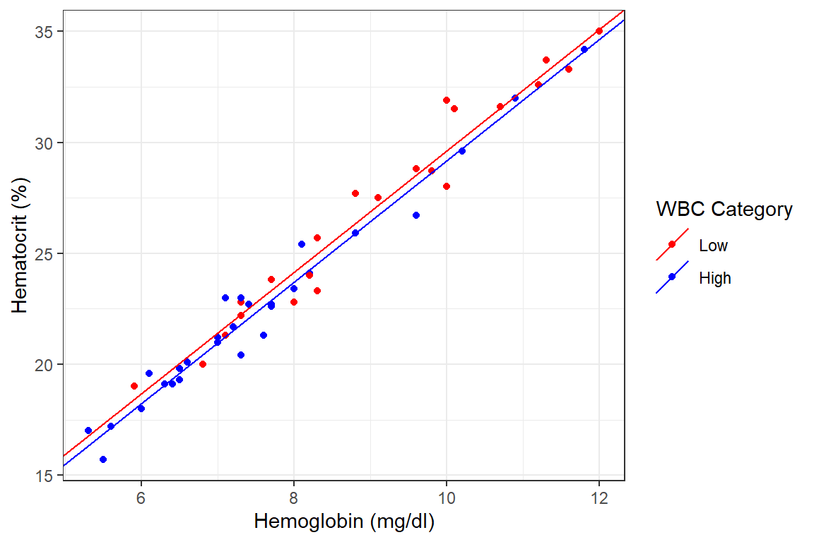
For both lines, the slope is the coefficient of hb. Thus the intercept for the “Low” wbc is 2.300622, that for the High wbc is \(2.300622 + -0.435617 = 1.865005\) and the common slope for both lines 2.735240. This is represented graphically below
df_blood %>%
    ggplot() +
    geom_point(aes(x = hb, y = hct, col = wbc.cat))+
    geom_abline(
        aes(intercept = 2.300622, slope = 2.735240, col = "Low"),
        show.legend = T)+
    geom_abline(
        aes(intercept = 2.300622 + -0.435617, slope = 2.735240, col = "High"),
        show.legend = T) +
    labs(x = "Hemoglobin (mg/dl)", y = "Hematocrit (%)")+
    scale_color_manual(
        name = "WBC Category",
        values = c("Low" = "red", "High" = "blue")) +
    theme_bw()
Conclusion: From our data, the hct of persons with High WBC count is about 0.4% lower than those with Low WBC assuming the two rise at the same rate in both groups. This difference however is not statistically significantly different from 0 (p = 0.128). Thus we do not have enough evidence that there is a difference in the levels of hct depending on the level of one’s WBC.
20.5 Regression with continuous and categorical independent variables with interaction
In the analysis above we assumed the slopes of the two lines are the same. However, this is usually not the case. To determine the individual slopes as well as their intercepts we need a linear regression with an interaction term. For this analysis, we seek to answer the question:
Are the rate of rise in hct with every rise in hb significantly different for persons with High compared to those with Low WBC?.
Fitting this linear regression is done in R as below.
| term | estimate | std.error | statistic | p.value | conf.low | conf.high |
|---|---|---|---|---|---|---|
| (Intercept) | 1.94 | 1.05 | 1.84 | 0.0724 | -0.184 | 4.06 |
| hb | 2.78 | 0.115 | 24.2 | 8.06e-28 | 2.54 | 3.01 |
| wbc.catHigh | 0.196 | 1.34 | 0.146 | 0.885 | -2.51 | 2.9 |
| hb:wbc.catHigh | -0.076 | 0.158 | -0.481 | 0.633 | -0.394 | 0.242 |
Four coefficients are generated. The (Intercept) is the intercept for the “Low”
wbc group. The hb coefficient represents the slope for the line representing
those with “Low” wbc. The intercept for “High” WBC is the sum of (Intercept)
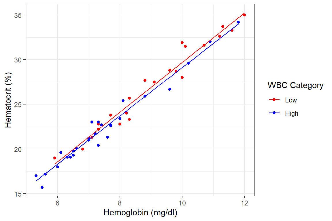
and wbc.catHigh (\(1.93925961 + 0.19624236 = 2.135502\)). Finally, the slope of
the regression line for “High” wbc is the sum of the coefficients hb and
hb:wbc.catHigh (\(2.77516971 + -0.07604741 = 2.699122\)).
This is graphically shown below
df_blood %>%
    ggplot(aes(x = hb, y = hct, color = wbc.cat))+
    geom_point()+
    geom_smooth(formula = y~x, se=FALSE, method = lm, size = .5)+
    theme_bw()+
    labs(x = "Hemoglobin (mg/dl)", y = "Hematocrit (%)")+
    scale_color_manual(
        name = "WBC Category",
        values = c("Low" = "red", "High" = "blue"))
Warning: Using `size` aesthetic for lines was deprecated in ggplot2
3.4.0.
ℹ Please use `linewidth` instead.
This warning is displayed once every 8 hours.
Call `lifecycle::last_lifecycle_warnings()` to see where
this warning was generated.
It is obvious from above that the slopes (rate of rise of hct concerninga unit rise in hb) are different for the two groups. That for the High WBC group is lower. However, is this decrease in the rate of rise a real effect or just a chance observation? To answer this question we need to use inferential statistics.
We now concern ourselves with the line hb:wbc.catHigh which indicates the
difference in slopes between the two. It appears the slope for the “High” wbc
group is about -0.076 (95%CI: -0.394 to 0.242, p=0.633) less than the “Low” wbc
group. This difference however is not statistically significant.
Conclusion: As the confidence interval contains the null value of 0 and the probability that this difference could have arisen by chance is relatively high (0.633), we conclude that we do not have significant evidence of a difference in slopes between those with “High” and “Low” WBCs.