8 Data Cleaning
Data to be analysed has to be ”cleaned” first of abnormal or invalid values. This should be done with the understanding of the data at hand, how it was collected in the first place and with very little prejudice or bias. This is a critical stage of the analysis where any arbitrary deletion or insertion of data could significantly alter the conclusions.
It, therefore, goes without saying that all modifications done at the data cleaning stage must have sound statistical, clinical as well as commonsensical reasons to it. Also, the whole process of data cleaning should be well documented and appropriately stored for future reference. In this regard, it is not good practice to edit the data in software such as Microsoft Excel though it may appear easy and tempting. This is because such software does not keep an audit trail.
8.1 Data dictionary or codebook
For well-collected and managed data, there should always be a dictionary. The dictionary outlines for every variable in the dataset its variable name, the meaning of the variable, the source of the variable (from the questionnaire, data collection sheet, etc.), the valid ranges or codes and the format. This is an invaluable tool for determining wrong and abnormal entries. It is also sometimes referred to as the codebook.
A typical example is the one below. This is the data dictionary for the blood_donors_3.dta file we are going to use.

8.2 Importing the data into R
The first step in analysis is to read or import the data into the data analysis
software where a general overview can be obtained. We begin by importing the
blood_donors_3.dta into R and calling it blood3.
blood3 <- readxl::read_xls("./Data/blood_donors_2.xls")8.3 Visualising the data in R
Next, we visualize the data
blood3
# A tibble: 25 × 6
      id    hb   hct   sex bldgrp pdonor
   <dbl> <dbl> <dbl> <dbl>  <dbl>  <dbl>
 1     1 10.5   31.8     1      3      3
 2     2 11.9   37.2     1      4      0
 3     3  1     26       1      1      1
 4     4  8.90  26.8     1      1      3
 5     5  7.80  24.2     1      1      2
 6     6 10     30.9     1      2      1
 7     7 10.4   33.9     1      2      0
 8     8 11.3   35       1      3      1
 9     9 16.4   NA       1      4      1
10    10 14.4   43.6     1      4      1
# ℹ 15 more rows
To visualise all the data we can use the print() or View() functions. Note
that this might not be the best if you have relatively big data. Below I
use the as.data.frame() function to display the whole data.
blood3 %>% as.data.frame()
   id   hb  hct sex bldgrp pdonor
1   1 10.5 31.8   1      3      3
2   2 11.9 37.2   1      4      0
3   3  1.0 26.0   1      1      1
4   4  8.9 26.8   1      1      3
5   5  7.8 24.2   1      1      2
6   6 10.0 30.9   1      2      1
7   7 10.4 33.9   1      2      0
8   8 11.3 35.0   1      3      1
9   9 16.4   NA   1      4      1
10 10 14.4 43.6   1      4      1
11 11 11.2 33.2   0      3     99
12 12 11.5 35.5   0      3      1
13 13 10.5 33.7   0      3      2
14 14 12.2 36.8   0      4      1
15 14 16.4 48.8   0      5      2
16 16 12.7 99.0   0      4      0
17 17  9.8 30.5   0      1      4
18 18 10.9 33.8   0      3      0
19 19 11.6 35.4   0      3      3
20 20 10.6 34.9   0      9      2
21 21  9.1 28.0   9      1      3
22 22 11.9 36.1   9      4      3
23 23 10.5 34.2   9      3      2
24 24 12.3 38.2   9      4      2
25 25 11.0 35.7   9      3      2
8.4 Describing or summarizing the data
We first use the glimpse() function to have a basic view of variable names and variable types
blood3 %>% glimpse()
Rows: 25
Columns: 6
$ id     <dbl> 1, 2, 3, 4, 5, 6, 7, 8, 9, 10, 11, 12, 13, …
$ hb     <dbl> 10.5, 11.9, 1.0, 8.9, 7.8, 10.0, 10.4, 11.3…
$ hct    <dbl> 31.8, 37.2, 26.0, 26.8, 24.2, 30.9, 33.9, 3…
$ sex    <dbl> 1, 1, 1, 1, 1, 1, 1, 1, 1, 1, 0, 0, 0, 0, 0…
$ bldgrp <dbl> 3, 4, 1, 1, 1, 2, 2, 3, 4, 4, 3, 3, 3, 4, 5…
$ pdonor <dbl> 3, 0, 1, 3, 2, 1, 0, 1, 1, 1, 99, 1, 2, 1, …
We can also use the dfSummary() function from the summarytools package to
give a more comprehensive output for each variable.
blood3 %>% summarytools::dfSummary()
Data Frame Summary
blood3
Dimensions: 25 x 6
Duplicates: 0

--------------------------------------------------------------------------------------------------------
No   Variable    Stats / Values            Freqs (% of Valid)   Graph               Valid      Missing
---- ----------- ------------------------- -------------------- ------------------- ---------- ---------
1    id          Mean (sd) : 13 (7.4)      24 distinct values   : : : : :           25         0
     [numeric]   min < med < max:                               : : : : :           (100.0%)   (0.0%)
                 1 < 13 < 25                                    : : : : :
                 IQR (CV) : 12 (0.6)                            : : : : :
                                                                : : : : :

2    hb          Mean (sd) : 11 (2.9)      21 distinct values             :         25         0
     [numeric]   min < med < max:                                         :         (100.0%)   (0.0%)
                 1 < 11 < 16.4                                            :
                 IQR (CV) : 1.5 (0.3)                                   . :
                                                                .     . : : : . :

3    hct         Mean (sd) : 36.8 (14.3)   24 distinct values     :                 24         1
     [numeric]   min < med < max:                                 :                 (96.0%)    (4.0%)
                 24.2 < 34.6 < 99                                 :
                 IQR (CV) : 4.7 (0.4)                             :
                                                                : : .         .

4    sex         Mean (sd) : 2.2 (3.5)     0 : 10 (40.0%)       IIIIIIII            25         0
     [numeric]   min < med < max:          1 : 10 (40.0%)       IIIIIIII            (100.0%)   (0.0%)
                 0 < 1 < 9                 9 :  5 (20.0%)       IIII
                 IQR (CV) : 1 (1.6)

5    bldgrp      Mean (sd) : 3.1 (1.7)     1 : 5 (20.0%)        IIII                25         0
     [numeric]   min < med < max:          2 : 2 ( 8.0%)        I                   (100.0%)   (0.0%)
                 1 < 3 < 9                 3 : 9 (36.0%)        IIIIIII
                 IQR (CV) : 2 (0.5)        4 : 7 (28.0%)        IIIII
                                           5 : 1 ( 4.0%)
                                           9 : 1 ( 4.0%)

6    pdonor      Mean (sd) : 5.6 (19.5)    0 : 4 (16.0%)        III                 25         0
     [numeric]   min < med < max:          1 : 7 (28.0%)        IIIII               (100.0%)   (0.0%)
                 0 < 2 < 99                2 : 7 (28.0%)        IIIII
                 IQR (CV) : 2 (3.5)        3 : 5 (20.0%)        IIII
                                           4 : 1 ( 4.0%)
                                           99 : 1 ( 4.0%)
--------------------------------------------------------------------------------------------------------
8.5 Cleaning individual variables
We note that all the variables are of type “double”. sex and bldgrp
however, should be factors. This is done and subsequently summarized below.
blood3 <-
    blood3 %>%
    mutate(sex = factor(sex,
                        levels = c(0,1,9),
                        labels = c("Female", "Male", "Missing")),
           bldgrp= factor(bldgrp,
                          levels = c(1, 2, 3, 4, 9),
                          labels = c("A", "B", "O", "AB", "Missing")))

blood3 %>% summarytools::dfSummary()
Data Frame Summary
blood3
Dimensions: 25 x 6
Duplicates: 0

--------------------------------------------------------------------------------------------------------
No   Variable    Stats / Values            Freqs (% of Valid)   Graph               Valid      Missing
---- ----------- ------------------------- -------------------- ------------------- ---------- ---------
1    id          Mean (sd) : 13 (7.4)      24 distinct values   : : : : :           25         0
     [numeric]   min < med < max:                               : : : : :           (100.0%)   (0.0%)
                 1 < 13 < 25                                    : : : : :
                 IQR (CV) : 12 (0.6)                            : : : : :
                                                                : : : : :

2    hb          Mean (sd) : 11 (2.9)      21 distinct values             :         25         0
     [numeric]   min < med < max:                                         :         (100.0%)   (0.0%)
                 1 < 11 < 16.4                                            :
                 IQR (CV) : 1.5 (0.3)                                   . :
                                                                .     . : : : . :

3    hct         Mean (sd) : 36.8 (14.3)   24 distinct values     :                 24         1
     [numeric]   min < med < max:                                 :                 (96.0%)    (4.0%)
                 24.2 < 34.6 < 99                                 :
                 IQR (CV) : 4.7 (0.4)                             :
                                                                : : .         .

4    sex         1. Female                 10 (40.0%)           IIIIIIII            25         0
     [factor]    2. Male                   10 (40.0%)           IIIIIIII            (100.0%)   (0.0%)
                 3. Missing                 5 (20.0%)           IIII

5    bldgrp      1. A                      5 (20.8%)            IIII                24         1
     [factor]    2. B                      2 ( 8.3%)            I                   (96.0%)    (4.0%)
                 3. O                      9 (37.5%)            IIIIIII
                 4. AB                     7 (29.2%)            IIIII
                 5. Missing                1 ( 4.2%)

6    pdonor      Mean (sd) : 5.6 (19.5)    0 : 4 (16.0%)        III                 25         0
     [numeric]   min < med < max:          1 : 7 (28.0%)        IIIII               (100.0%)   (0.0%)
                 0 < 2 < 99                2 : 7 (28.0%)        IIIII
                 IQR (CV) : 2 (3.5)        3 : 5 (20.0%)        IIII
                                           4 : 1 ( 4.0%)
                                           99 : 1 ( 4.0%)
--------------------------------------------------------------------------------------------------------
8.6 Checking for duplicated records
We begin official data cleaning by checking if we have duplicate records in our data
8.7 Cleaning individual variables
Next, we begin to sort the variables one by one. We begin with the study id variable. We begin by looking for duplicated study ids.
blood3 %>% janitor::get_dupes(id)
# A tibble: 2 × 7
     id dupe_count    hb   hct sex    bldgrp pdonor
  <dbl>      <int> <dbl> <dbl> <fct>  <fct>   <dbl>
1    14          2  12.2  36.8 Female AB          1
2    14          2  16.4  48.8 Female <NA>        2
Study id 14 is duplicated! Next, we visually inspect the study ids
It looks like the study ids are in numeric order from 1 to 25 but 14 is duplicated while 15 is missing. We solve this by writing a new study id variable. Afterwards, we check to see if there are any more duplicates.
blood3 <-
    blood3 %>%
    mutate(id = 1:25)

blood3 %>% janitor::get_dupes(id)
No duplicate combinations found of: id
# A tibble: 0 × 7
# ℹ 7 variables: id <int>, dupe_count <int>, hb <dbl>,
#   hct <dbl>, sex <fct>, bldgrp <fct>, pdonor <dbl>
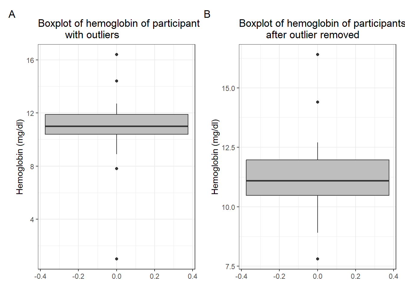
Next, we inspect the hb variable with a summary and a boxplot. We observe from
the summary none of the haemoglobin observations is missing. The boxplot of
the hb is as shown in A below. We observe 4 are outliers and one looks very
extreme.
A <-
    blood3 %>%
    ggplot(aes(y = hb)) +
    geom_boxplot(fill = "grey") +
    labs(y = "Hemoglobin (mg/dl)",
         title = "Boxplot of hemoglobin of participants
         with outliers") +
    theme_bw()
We convert this observation to missing as below.
blood3 <-
    blood3 %>%
    mutate(hb = ifelse(hb < 4, NA, hb))
B <-
blood3 %>%
ggplot(aes(y = hb)) +
geom_boxplot(fill = "grey") +
labs(y = "Hemoglobin (mg/dl)",
title = "Boxplot of hemoglobin of participants
after outlier removed") +
theme_bw()
A + B + plot_annotation(tag_levels = 'A')
Warning: Removed 1 rows containing non-finite values
(`stat_boxplot()`).
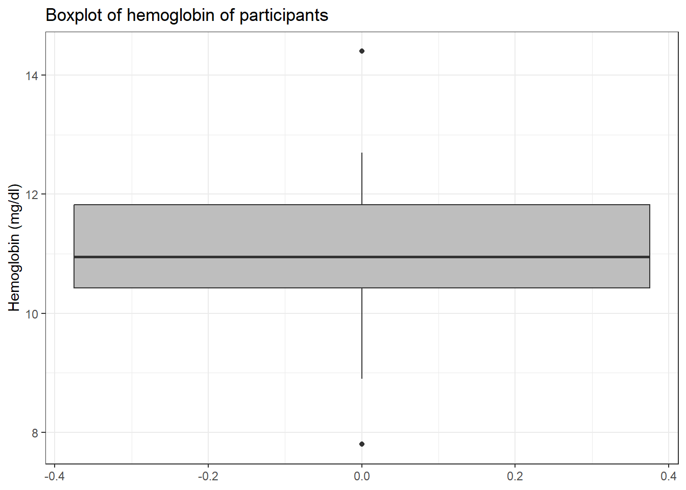
And redraw the boxplot without the outlier.
blood3 %>%
    drop_na() %>%
    ggplot(aes(y = hb)) +
    geom_boxplot(fill ="grey") +
    labs(y = "Hemoglobin (mg/dl)",
         title = "Boxplot of hemoglobin of participants") +
    theme_bw()
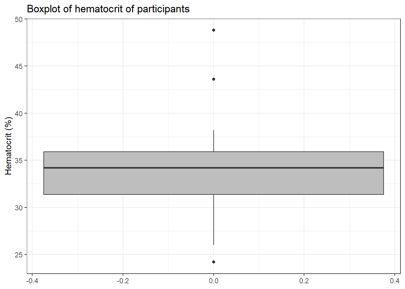
Next, we focus on the hct variable. It is of note that it has 99 which represents ‘missing’. We
therefore remove that as below
blood3 <-
    blood3 %>%
    mutate(hct = ifelse(hct >90, NA, hct))
And draw the boxplot below
blood3 %>%
    drop_na(hct) %>%
    ggplot(aes(y = hct)) +
    geom_boxplot(fill = "grey")+
    labs(y = "Hematocrit (%)",
         title = "Boxplot of hematocrit of participants") +
    theme_bw()
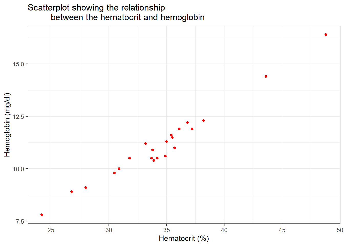
Because we know the hematocrit has a relationship with the haemoglobin, we use a scatter plot to visualise and possibly pick up suspicious data.
blood3 %>%
    drop_na(hb, hct) %>%
    ggplot(aes(x = hct, y = hb)) +
    geom_point(col = "red") +
    labs(x = "Hematocrit (%)",
         y = "Hemoglobin (mg/dl)",
         title = "Scatterplot showing the relationship
         between the hematocrit and hemoglobin")+
    theme_bw()
Next, we inspect the sex variable
We then convert the “Missing” category to NA
blood3 <-
    blood3 %>%
    mutate(sex = fct_recode(sex, NULL = "Missing"))
And then check
Next, we sort out the bldgrp variable
blood3 %>%
    count(bldgrp)
# A tibble: 6 × 2
  bldgrp      n
  <fct>   <int>
1 A           5
2 B           2
3 O           9
4 AB          7
5 Missing     1
6 <NA>        1
We convert Missing to NA and visualize the variable
blood3 <-
    blood3 %>%
    mutate(bldgrp = fct_recode(bldgrp, NULL = "Missing"))

blood3 %>% count(bldgrp)
# A tibble: 5 × 2
  bldgrp     n
  <fct>  <int>
1 A          5
2 B          2
3 O          9
4 AB         7
5 <NA>       2
Next, we sort out the pdonor
blood3 <-
    blood3 %>%
    mutate(pdonor = ifelse(pdonor == 99, NA, pdonor))
8.8 Visualising the cleaned data
Finally, we summarize the data below
blood3 %>%
    summarytools::dfSummary()
Data Frame Summary
blood3
Dimensions: 25 x 6
Duplicates: 0

--------------------------------------------------------------------------------------------------
No   Variable    Stats / Values           Freqs (% of Valid)   Graph          Valid      Missing
---- ----------- ------------------------ -------------------- -------------- ---------- ---------
1    id          Mean (sd) : 13 (7.4)     25 distinct values   : : : : :      25         0
     [integer]   min < med < max:         (Integer sequence)   : : : : :      (100.0%)   (0.0%)
                 1 < 13 < 25                                   : : : : :
                 IQR (CV) : 12 (0.6)                           : : : : :
                                                               : : : : :

2    hb          Mean (sd) : 11.4 (2)     20 distinct values       :          24         1
     [numeric]   min < med < max:                                  :          (96.0%)    (4.0%)
                 7.8 < 11.1 < 16.4                                 :
                 IQR (CV) : 1.5 (0.2)                            . :
                                                               . : : : . :

3    hct         Mean (sd) : 34.1 (5.4)   23 distinct values       :          23         2
     [numeric]   min < med < max:                                  : .        (92.0%)    (8.0%)
                 24.2 < 34.2 < 48.8                                : :
                 IQR (CV) : 4.6 (0.2)                            . : :
                                                               . : : : . .

4    sex         1. Female                10 (50.0%)           IIIIIIIIII     20         5
     [factor]    2. Male                  10 (50.0%)           IIIIIIIIII     (80.0%)    (20.0%)

5    bldgrp      1. A                     5 (21.7%)            IIII           23         2
     [factor]    2. B                     2 ( 8.7%)            I              (92.0%)    (8.0%)
                 3. O                     9 (39.1%)            IIIIIII
                 4. AB                    7 (30.4%)            IIIIII

6    pdonor      Mean (sd) : 1.7 (1.1)    0 : 4 (16.7%)        III            24         1
     [numeric]   min < med < max:         1 : 7 (29.2%)        IIIII          (96.0%)    (4.0%)
                 0 < 2 < 4                2 : 7 (29.2%)        IIIII
                 IQR (CV) : 1.2 (0.7)     3 : 5 (20.8%)        IIII
                                          4 : 1 ( 4.2%)
--------------------------------------------------------------------------------------------------
8.9 Generating new variables
Often after cleaning individual variables a data analyst will be required to generate new variables from the old ones. We will put this into practice by generating the presence of Anemia if the hb is less than 11g/dl.
blood3 <-
    blood3 %>%
    mutate(anemia = case_when(hb < 11 ~ "Yes", hb >= 11 ~ "No") %>% factor())

summarytools::dfSummary(blood3)
Data Frame Summary
blood3
Dimensions: 25 x 7
Duplicates: 0

--------------------------------------------------------------------------------------------------
No   Variable    Stats / Values           Freqs (% of Valid)   Graph          Valid      Missing
---- ----------- ------------------------ -------------------- -------------- ---------- ---------
1    id          Mean (sd) : 13 (7.4)     25 distinct values   : : : : :      25         0
     [integer]   min < med < max:         (Integer sequence)   : : : : :      (100.0%)   (0.0%)
                 1 < 13 < 25                                   : : : : :
                 IQR (CV) : 12 (0.6)                           : : : : :
                                                               : : : : :

2    hb          Mean (sd) : 11.4 (2)     20 distinct values       :          24         1
     [numeric]   min < med < max:                                  :          (96.0%)    (4.0%)
                 7.8 < 11.1 < 16.4                                 :
                 IQR (CV) : 1.5 (0.2)                            . :
                                                               . : : : . :

3    hct         Mean (sd) : 34.1 (5.4)   23 distinct values       :          23         2
     [numeric]   min < med < max:                                  : .        (92.0%)    (8.0%)
                 24.2 < 34.2 < 48.8                                : :
                 IQR (CV) : 4.6 (0.2)                            . : :
                                                               . : : : . .

4    sex         1. Female                10 (50.0%)           IIIIIIIIII     20         5
     [factor]    2. Male                  10 (50.0%)           IIIIIIIIII     (80.0%)    (20.0%)

5    bldgrp      1. A                     5 (21.7%)            IIII           23         2
     [factor]    2. B                     2 ( 8.7%)            I              (92.0%)    (8.0%)
                 3. O                     9 (39.1%)            IIIIIII
                 4. AB                    7 (30.4%)            IIIIII

6    pdonor      Mean (sd) : 1.7 (1.1)    0 : 4 (16.7%)        III            24         1
     [numeric]   min < med < max:         1 : 7 (29.2%)        IIIII          (96.0%)    (4.0%)
                 0 < 2 < 4                2 : 7 (29.2%)        IIIII
                 IQR (CV) : 1.2 (0.7)     3 : 5 (20.8%)        IIII
                                          4 : 1 ( 4.2%)

7    anemia      1. No                    13 (54.2%)           IIIIIIIIII     24         1
     [factor]    2. Yes                   11 (45.8%)           IIIIIIIII      (96.0%)    (4.0%)
--------------------------------------------------------------------------------------------------