16 Confounding and Interaction
16.1 Introduction
A new waiter employed in a bar to serve ice in glasses in Accra made an
observation which seem irrational. He realized that customers who he served
ice often ended up drunk. He is the first to accept this does not make sense but
strongly believe he is right. He approached a friend who is a researcher and
they both decided to investigate this. The friend decided to take data on 510
randomly selected customers. This data is recorded in drinks.txt.
The variables collected include id the sequentially allocated study id, sex,
sex of the customer, liquor whether the customer took an alcoholic liquor
(spirits, brandy, etc), ice whether the customer was served ice in a glass,
drunk whether the customer ended up being drunk, food whether the customer
was served food and age, age in years of the customer. The task now is to
determine from the data if ingesting ice is associated with being drunk.
16.2 Effect and effect size
16.2.1 Effect
Before we begin to discuss the above problem we first look at what in statistical terms is meant by effect. The effect is defined as a change that occurs as a consequence of an action. In statistical terms, the effect is usually the change in one variable by another. For instance, the effect could be the mean change in blood pressure (effect) after taking a drug (the action). Two of the most common ways of expressing effect in categorical data analysis are the odds ratio (OR) and Relative Risk (RR). These two usually determine the effect by comparing the odds or risk in two groups and expressing the effect as the ratios.
16.2.2 Effect size
It does not only suffice to report the effect but also its size. People would want to know not only if an intervention makes a difference but also how much difference it makes. Effect size can be in the opposite direction. For instance, the difference between the blood pressure after taking a medication may be positive (when the pressure after taking the drug is more than before taking) or negative (when the pressure becomes less when the drug is taken). On the other hand, effects can be on the same side but with a difference in magnitude. An OR of 5.1 is much higher than 1.5 despite both indicating increased odds of having the outcome. We are going to apply this notion in determining confounders and effect modifiers.
Now back to the waiter’s issue. First, we read the data.
df_drinks <-
    read.table("./Data/drinks.txt", header=T, sep="\t") %>%
    mutate(
        across(
            c(liquor, ice, drunk, food),
            ~factor(.x, levels = c(0,1), labels = c("No","Yes"))
        ),
        sex = factor(sex)
    )
And then summarize the data
options(huxtable.knit_print_df = FALSE)
df_drinks %>%
    summarytools::dfSummary(graph.col = F)
Data Frame Summary
df_drinks
Dimensions: 510 x 7
Duplicates: 0

---------------------------------------------------------------------------------------
No   Variable    Stats / Values              Freqs (% of Valid)    Valid      Missing
---- ----------- --------------------------- --------------------- ---------- ---------
1    id          Mean (sd) : 255.5 (147.4)   510 distinct values   510        0
     [integer]   min < med < max:            (Integer sequence)    (100.0%)   (0.0%)
                 1 < 255.5 < 510
                 IQR (CV) : 254.5 (0.6)

2    sex         1. Female                   256 (50.2%)           510        0
     [factor]    2. Male                     254 (49.8%)           (100.0%)   (0.0%)

3    liquor      1. No                       155 (30.4%)           510        0
     [factor]    2. Yes                      355 (69.6%)           (100.0%)   (0.0%)

4    ice         1. No                       191 (37.5%)           510        0
     [factor]    2. Yes                      319 (62.5%)           (100.0%)   (0.0%)

5    drunk       1. No                       186 (36.5%)           510        0
     [factor]    2. Yes                      324 (63.5%)           (100.0%)   (0.0%)

6    age         Mean (sd) : 35.8 (5.1)      31 distinct values    510        0
     [integer]   min < med < max:                                  (100.0%)   (0.0%)
                 19 < 36 < 51
                 IQR (CV) : 7 (0.1)

7    food        1. No                       288 (56.5%)           510        0
     [factor]    2. Yes                      222 (43.5%)           (100.0%)   (0.0%)
---------------------------------------------------------------------------------------

options(huxtable.knit_print_df = TRUE)
In this section, we make use of two main functions cc() and mhor() from the
epicalc package. First, we determine the effect of having ice concerning
being drunk by using the odds ratio.
df_drinks %$% epiDisplay::cc(drunk, ice)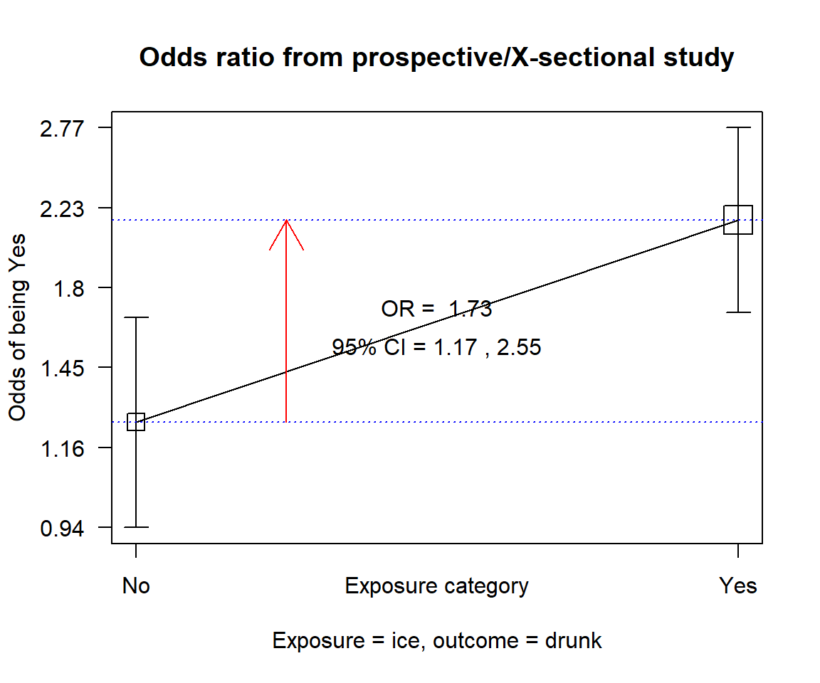
       ice
drunk    No Yes Total
  No     85 101   186
  Yes   106 218   324
  Total 191 319   510

OR =  1.73
95% CI =  1.2, 2.51
Chi-squared = 8.5, 1 d.f., P value = 0.004
Fisher's exact test (2-sided) P value = 0.004
It appears the waiter is right! Taking ice is associated with significantly higher odds of getting drunk (OR: 1.73, 95% CI: 1.17 to 2.55, p<.001). This we all agree defies logic. The question then is: How did this arise?
16.2.3 Confounding
In research there often arises the situation where the observed effect of a variable tends to depend on another. For instance, in our case, the effect of ice on making customers drunk could be because it is associated with another item. If customers who took ice also took in some hard liquor at the same time this may make it seem that taking ice is associated with being drunk. This would be a typical case of confounding with the liquor ingestion confounding the effect of ice.
For a variable to be a confounder it must meet these basic properties
- The confounder must be related to the exposure (ice) variable
- The confounder must be related to the outcome (drunk) variable
- The confounder should not be on the causal pathway between the exposure(ice) and outcome (drunk).
The first two conditions are easily tested statistically but the last can only be tested with prior knowledge, often coming from epidemiological and scientific facts. The investigator of the bar study suspects liquor to be a confounder to the effect of ice so sets out to determine this. First, he looks out for the relationship between the suspected confounder and the outcome
df_drinks %$% epiDisplay::cc(drunk, liquor)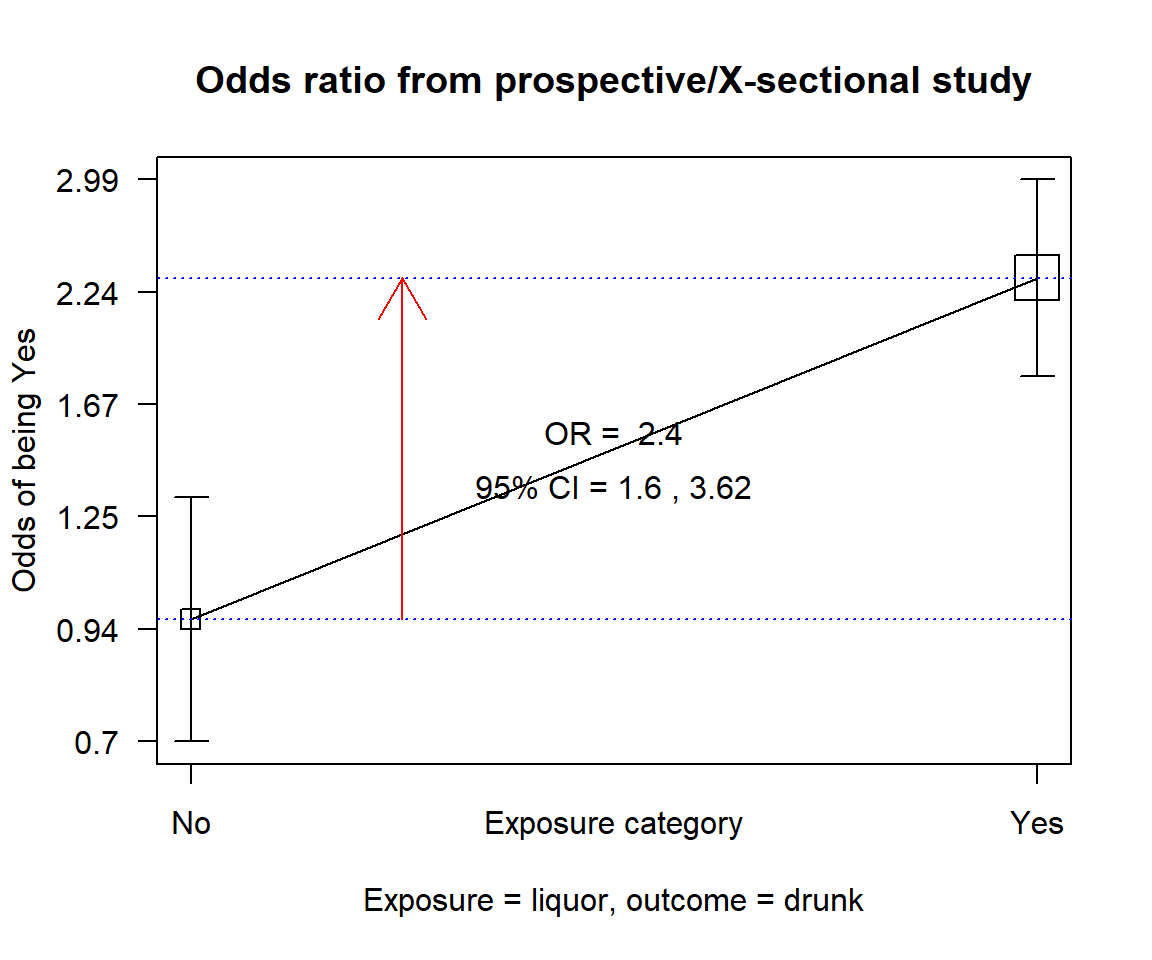
       liquor
drunk    No Yes Total
  No     79 107   186
  Yes    76 248   324
  Total 155 355   510

OR =  2.41
95% CI =  1.63, 3.55
Chi-squared = 20.2, 1 d.f., P value = 0
Fisher's exact test (2-sided) P value = 0
Having liquor is strongly associated with being drunk with an OR = 2.41 (95%CI: 1.6, 3.62, p<.001). Next, we test the association between the exposure and the possible confounder.
df_drinks %$% epiDisplay::cc(ice, liquor, graph = F)

       liquor
ice      No Yes Total
  No    120  71   191
  Yes    35 284   319
  Total 155 355   510

OR =  13.71
95% CI =  8.68, 21.67
Chi-squared = 151.85, 1 d.f., P value = 0
Fisher's exact test (2-sided) P value = 0
There is a strong association between having ice and taking hard liquor (OR: 13.71, 95% CI: 8.48 to 22.33, p<.001). With this relationship established the first two conditions stated above have been fulfilled.
Our next task is to determine if the consumption of liquor is a confounder of the effect of ice. We do this by determining the adjusted OR and comparing it to the crude OR (unadjusted OR). We recall from above that the crude OR is 1.73 (95% CI = 1.17 to 2.55, p=0.004). The Mantel-Haenszel odd ratios determined by the mhor() function is an OR adjusted for the possible confounder. This is shown below
df_drinks %$% epiDisplay::mhor(drunk, ice, liquor)

Stratified analysis by  liquor
               OR lower lim. upper lim. P value
liquor No    1.13      0.497       2.58   0.848
liquor Yes   1.14      0.621       2.05   0.666
M-H combined 1.14      0.726       1.78   0.574

M-H Chi2(1) = 0.32 , P value = 0.574
Homogeneity test, chi-squared 1 d.f. = 0 , P value = 0.986 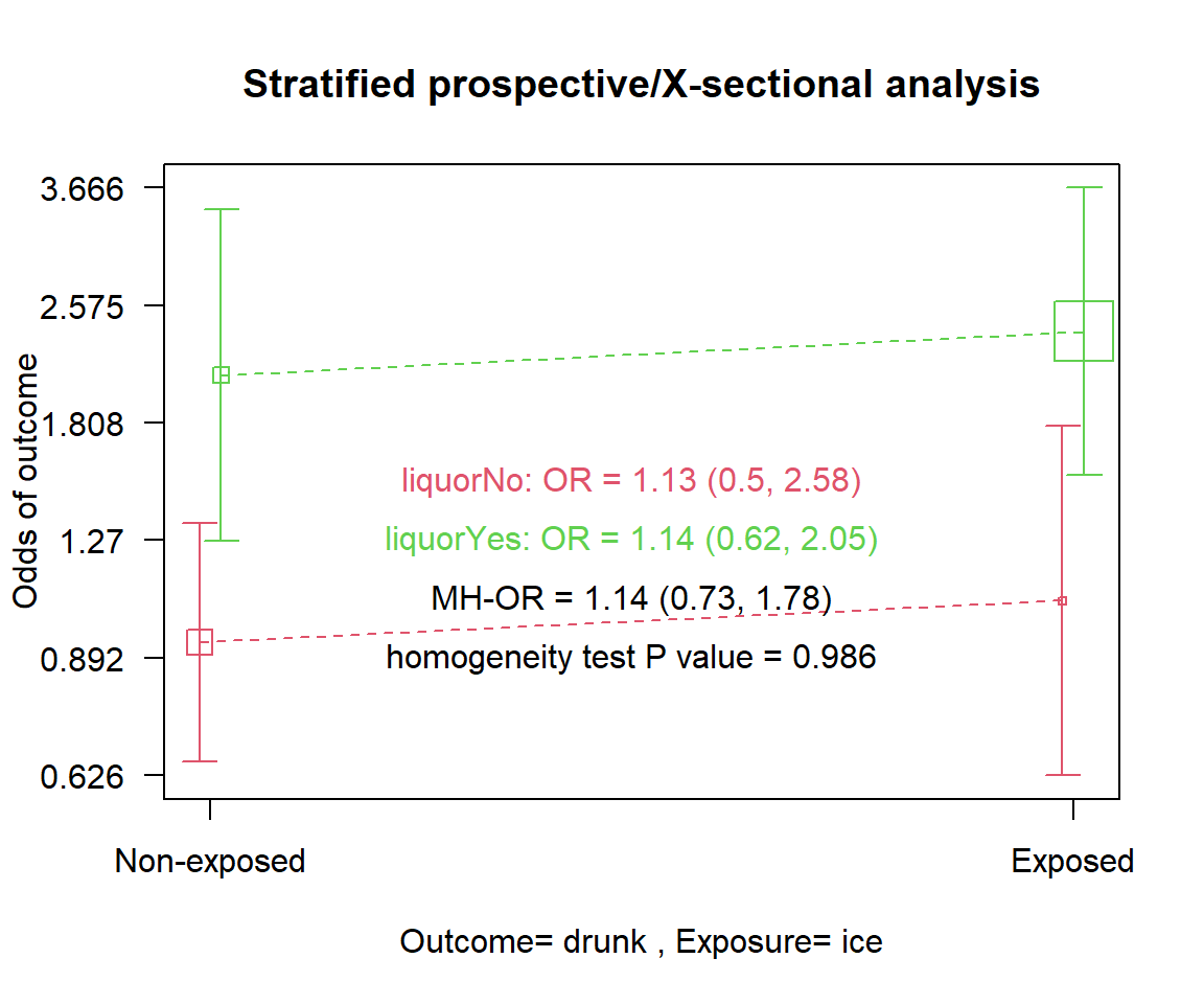
The function first stratifies the odds of getting drunk after taking ice into the individual groups of the possible confounding variable. It then determines the OR for each level of the confounder, 1.14(95%CI= 0.621 to 2.05, p=0.666) for those who took liquor and 1.13 (95%CI: 0.497 to 2.58, p=0.848) for those who did not. It then reports the MH combined (adjusted) OR of 1.14 (95%CI: 0.726 to 1.78, p=0.574). Thus stratification or adjustment has reduced the OR or effect of ice from a significant 1.7 to a non-significant relationship 1.1. The effect has all but disappeared as ice is no longer significantly associated with getting drunk after adjustment. This shows that ice on its own does not cause people to be drunk and the observed effect was just an issue of confounding by the consumption of liquor.
Above we have shown the relationship between the three variables involved in demonstrating the confounding effect of liquor on the effect of taking ice. We can then ask: Is ice a confounder to the relationship between being drunk and consumption of liquor? Remember the crude OR for this effect is 2.41 (95%CI: 1.6, 3.62, p<.001). To answer the question we determine the adjusted OR below.
df_drinks %$% epiDisplay::mhor(drunk, liquor, ice)

Stratified analysis by  ice
               OR lower lim. upper lim.  P value
ice No       2.22       1.16       4.33 0.010714
ice Yes      2.24       1.03       4.86 0.032828
M-H combined 2.24       1.41       3.56 0.000589

M-H Chi2(1) = 11.81 , P value = 0.001
Homogeneity test, chi-squared 1 d.f. = 0 , P value = 0.981 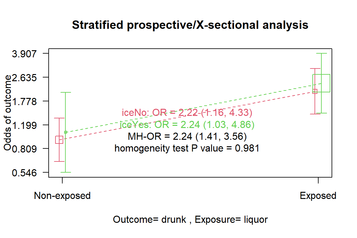
The output shows that the adjusted OR (OR=2.24, 95%CI: 1.41 to 3.56, p<.001) is barely different from the crude OR and also retains its significant effect. The consumption of ice is therefore not a confounder to the effect of hard liquor.
In summary to determine if a variable is a confounder we need to determine its association with the exposure and outcome variable. If there is an association we then determine the crude effect and adjusted effect. If these two are significantly different then we can conclude the presence of a confounder.
However, the definition of “significant effect” is always difficult to determine. Some say a change in at least 10% of the crude effect can be considered enough. Whenever there is a possible confounder the adjusted effect should be reported. Also, it is worth noting that effect change could be making the effect higher or lower. A confounder that for instance results in a crude OR of 2.4 and an adjusted OR of 1.5 is a positive confounder while one that has a crude OR of 1.5 but adjusted OR of 2.5 shows negative confounding.
16.3 Interaction or Effect modification
It is common knowledge among those who drink alcoholic beverages that filling your tummy with food often delays getting drunk when one consumes alcoholic beverages. The investigator of the bar data now wants to determine if this is so. If this notion is right then getting drunk after taking hard liquor should be dependent on whether the customer also ordered and ate some food as well. This is a typical example of effect modification (a term often used by epidemiologists) or interaction (used by statisticians). The two essentially means the same. By definition, effect modification occurs when the effect size of an exposure (liquor) on an outcome (drunk) differs depending on the level of a third variable (eating food). When this occurs just computing and reporting the overall effect is misleading.
We begin our investigation for food causing an interaction in the effect of drinking hard liquor by determining the OR of getting drunk when one took some food and when one didn’t.
We begin with those who ate some food.
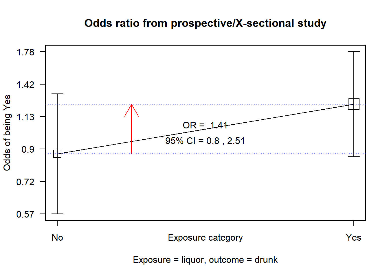
       liquor
drunk    No Yes Total
  No     47  60   107
  Yes    41  74   115
  Total  88 134   222

OR =  1.41
95% CI =  0.82, 2.43
Chi-squared = 1.59, 1 d.f., P value = 0.208
Fisher's exact test (2-sided) P value = 0.219
There is a statistically insignificant odds of getting drunk after taking hard liquor when one eats as well with an OR 1.41 (95% CI: 0.8 to 2.51, p=0.208). Next, we do the same for those who did not eat
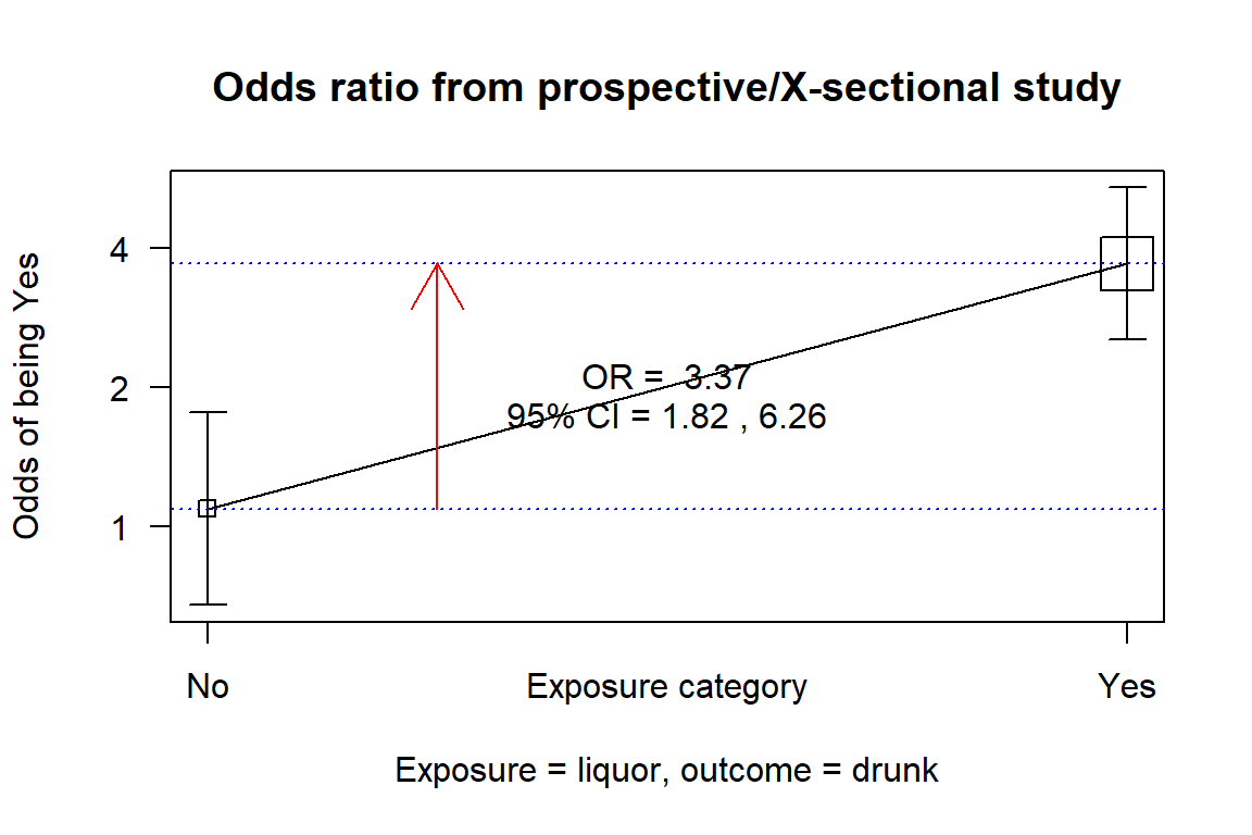
       liquor
drunk    No Yes Total
  No     32  47    79
  Yes    35 174   209
  Total  67 221   288

OR =  3.38
95% CI =  1.9, 6.03
Chi-squared = 18.13, 1 d.f., P value = 0
Fisher's exact test (2-sided) P value = 0
The OR of getting drunk if one takes liquor and on an empty stomach is much
higher and statistically significant (OR: 3.38, 95% CI: 1.82 to 6.26, p<.001).
We seem to have quite a substantial difference in the effect of drinking liquor
depending on food intake or not. To be sure if this food intake is a significant
effect modifier we subject this to a formal test using the mhor() function.
df_drinks %$% epiDisplay::mhor(drunk, liquor, food, graph = F)

Stratified analysis by  food
               OR lower lim. upper lim.  P value
food No      3.37      1.817       6.26 4.16e-05
food Yes     1.41      0.795       2.51 2.19e-01
M-H combined 2.08      1.406       3.09 1.78e-04

M-H Chi2(1) = 14.05 , P value = 0
Homogeneity test, chi-squared 1 d.f. = 4.65 , P value = 0.031
The stratified analysis output above shows our prior calculated stratified ORs as well as the combined Mantel-Haenszel OR. The Homogeneity test above tests the null hypothesis:
H0: There is no difference between the two stratified Odds ratios.
A p-value of 0.031, therefore, indicates a statistically significant difference in effects (OR) for those who ate and those who did not. We, therefore, conclude that there is significant interaction between food intake and getting drunk if one takes hard liquor.
In this section, we have dealt with detecting a confounder or interaction variable in categorical data analysis. This is just scratching the surface. In subsequent chapters, we would be dealing a lot more with these but using regression analysis.